Agentic Search Is Not Enough: Why AI Agents Need a Context Graph

TL;DR

Agentic search can help agents find information, but it cannot give them a durable model of how an organization’s systems relate. Without a persistent representation of entities, relationships, and history, agents have to rebuild context from scattered systems every time they act.

A context graph gives agents a data model of the organization, a unified index across scattered systems, a memory layer for prior decisions, and a computational substrate for structural queries like key asset identification and impact analysis. This makes agents more effective, reliable, and efficient. They operate from a shared organizational state, reuse prior work, and leave behind memory future tasks can build on.

AI agents are transitioning from simple-task assistants to systems expected to perform long-running tasks across heterogeneous systems. To successfully execute complex tasks such as debugging a failed data pipeline or building a new AI model, an agent needs a unified view of how these disparate pieces connect.

The current industry default is to hand the agent more tools and hope for the best. While a capable agent can theoretically piece together context on the fly, constructing cross-system structure at runtime creates severe bottlenecks. Rebuilding that structure from scratch for every task is inefficient and error-prone. In addition, trying to recover complex historical sequences from scattered primary sources is simply too slow and brittle for real-time inference.

Waiting for larger context windows or smarter models won't solve this. An infinite context window doesn't help if the retrieved documents contradict each other and the agent has no way to verify which one is canonical. A stronger reasoning engine still can't deduce what a production database looked like during an incident three weeks ago if the APIs only return the current state. Model capability cannot replace missing data infrastructure.

The missing infrastructure layer is a context graph. Instead of forcing agents to write fragile, on-the-fly code to guess at relationships, a context graph replaces unpredictable exploratory loops with instant, deterministic structural lookups. It reconciles conflicting signals, keeps a permanent record to accurately reconstruct the past, and continuously learns from user interactions so it can dynamically self-heal. 

This post explains what a context graph is, how to construct one, how retrieval works, and why this infrastructure becomes strictly necessary when deploying agents for long-horizon work. To make the engineering trade-offs concrete, we will use a running example of an e-commerce company to demonstrate exactly where agentic search breaks down and where a shared graph is necessary.

What is a context graph?

A context graph is often described as a living record of decision traces, linked across entities and time so precedent becomes searchable. However, decision traces only become useful when they are connected to the surrounding context that gives them meaning: the data, code, documentation, executions, and organizational entities they relate to.

In most organizations, that context is distributed across warehouses, databases, repositories, dashboards, wikis, and operational tools. A context graph must reconcile those distributed representations, linking the same underlying entities, such as a seller, product, service, dataset, or model, even when they appear under different identifiers.

The systems vary, but the inputs usually fall into recurring categories:

• Structured data: Warehouse tables, transactional databases, object storage, feature stores, and vector stores.

• Code and configuration: Application code, pipeline code, infrastructure definitions, and service metadata.

• Documentation and institutional knowledge: Design docs, wikis, data dictionaries, and runbooks.

• Analytical artifacts: Dashboards, reports, queries, notebooks, and metric definitions.

• ML artifacts: Datasets, experiment runs, checkpoints, evaluations, and registry metadata.

• Collaboration records: Discussions, reviews, meeting notes, and decisions.

• Operational systems: Tickets, incidents, support cases, project trackers, and CRM records.

Each source contributes a partial view, such as structure, behavior, history, ownership, intent, or outcome. The value of a context graph comes from binding those views into one structure agents can reason over end to end.

Once connected, the graph serves four operational roles for agents:

• Data model: A representation of the organization’s entities, assets, workflows, owners, and relationships.

• Index: A lookup layer over distributed systems, helping agents find relevant tables, documents, services, dashboards, tickets, runs, and code without scanning each source independently.

• Memory layer: A record of prior decisions, changes, failures, experiments, and exceptions. Linked back to the surrounding context, that history becomes precedent agents can reuse, not scattered institutional memory.

• Computational substrate: A structure for queries that are hard to express as retrieval alone, including dependency tracing, blast-radius analysis, lineage traversal, ownership lookup, temporal comparison, and multi-hop reasoning.

Without a context graph, agents have to reconstruct this state at runtime from fragmented sources. Now, let's examine how this state gets built, which construction choices matter, and what changes when agents can rely on it.

A running example: an e-commerce company

We use an e-commerce company as a running example. The core business entities and relational structure come from Olist’s public Kaggle dataset. We then add surrounding systems, teams, and workflows to show how context graph construction and retrieval decisions play out in practice.

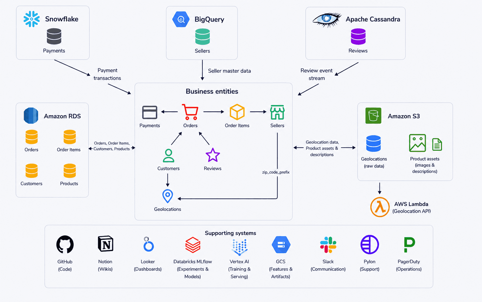
The figure above shows the company’s data and supporting systems. At the center are the business entities the company runs on: customers, orders, order items, reviews, sellers, products, payments, and geolocations. Those entities are materialized across multiple backend systems. RDS holds operational order, customer, and product data; Snowflake holds payment transactions; BigQuery is the source of truth for seller master data; Cassandra stores the review event stream; and S3 holds raw geolocation data and unstructured product assets such as images and free-text descriptions. Around those systems sit the tools that give the data operational meaning: GitHub for code, Notion for internal knowledge, Looker for dashboards, MLflow and Vertex AI for model development, Slack for collaboration, Pylon for support, and PagerDuty for incidents.

Different teams use overlapping slices of this context. The applications team builds the e-commerce platform that generates much of the data. Analytics maintains dashboards for sellers, products, and revenue. Data science works on forecasting. The ML team trains and serves the recommendation model. Each team could use agents for different tasks, but those agents are limited if they only see one system at a time.

A context graph for this company would link data assets, logical business entities, code, documentation, execution records, teams, and operational systems through relationships such as identity, dependency, ownership, lineage, usage, and runtime interaction. Its value is not the links themselves, but the structure they create. This structure provides a way for agents to move across systems, correlate evidence, distinguish declared intent from runtime behavior, and reason from a more complete view of operational reality.

Context graph construction

Constructing a context graph is not an exercise in making a perfectly clean representation of the organization. The graph needs to preserve enough evidence for agents to reason across systems, including partial evidence, ambiguous references, or stale documents. Completeness matters because evidence that looks low-value at ingestion time may become useful when linked to a future task, incident, model, or decision.

Construction alone, however, does not determine whether the system is effective. As with any database system, there is a trade-off between organizing information during ingestion and filtering it during retrieval. The graph can favor completeness at ingestion if evidence is stored with provenance, timestamps, and confidence metadata. Ranking, task-specific traversal, temporal filters, and confidence thresholds then determine what becomes visible for a particular agent task. A system can preserve noisy history, partial evidence, abandoned experiments, and stale documents without exposing all of it equally to every query.

However, there is a limit to how much retrieval can compensate. If construction is too loose, the graph becomes a bloated, hard-to-query collection of stale relationships and conflicting facts. Building a useful context graph comes down to four connected construction challenges: schema design, ingestion and versioning, entity resolution, and relationship accuracy.

There is no universal architecture for a context graph. The right design depends on the organization’s systems, scale, and retrieval patterns. In this case, our goal is to highlight the trade-offs behind each construction challenge and use the e-commerce company to show how those choices play out in practice.

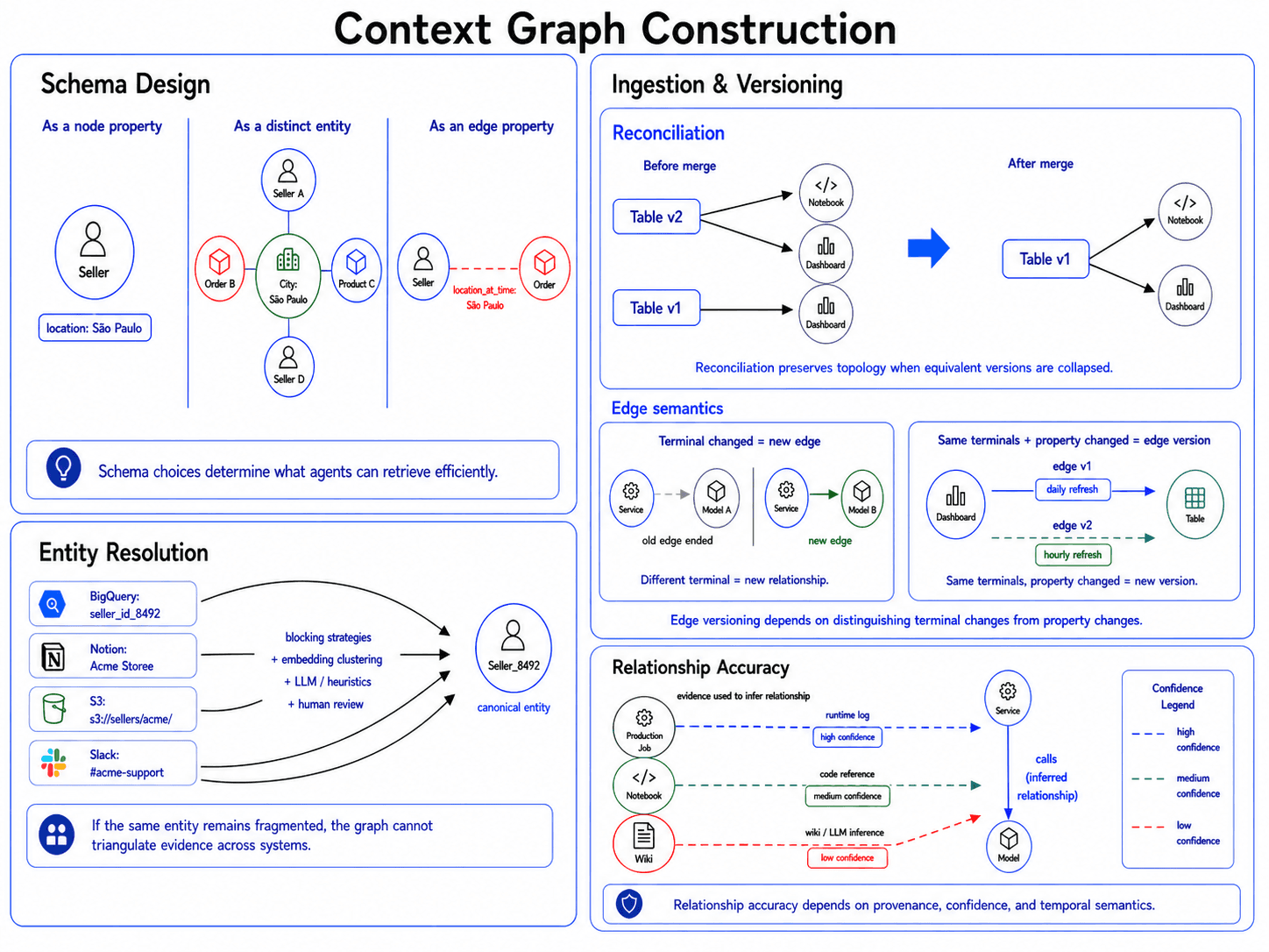
Schema design: defining the data model

Building the graph starts with a seemingly simple set of questions: what exactly is a node, what is a property, and what is an edge?

These choices determine what agents can retrieve cheaply and what will cause timeouts. Consider how the example e-commerce company might represent seller geolocations. There are three valid approaches:

1. As a node property. Store location directly on the seller node. This is compact and cheap when location is only seller metadata.

2. As a distinct entity. Make the city or region its own node. This costs an extra traversal but supports queries like “show me all sellers within 50 miles of São Paulo.”

3. As an edge property. Store location on the seller-order edge. This fits cases where location is contextual, time-varying, or specific to a transaction.

The same pattern shows up across the graph. Should columns be nodes or only tables? Should a model be a logical entity linked to checkpoints, registry entries, and deployments, or should each artifact stand on its own? Should dashboards and notebooks be represented as file-like assets, or as semantic objects with ownership, usage, and execution relationships?

Beyond just physical structure, schema design also dictates how derived metadata is stored. A raw database column node is useful, but its value multiplies when the schema allows for asynchronous enrichment, such as a background job attaching an is_PII=true tag or inheriting access control lists (ACLs) directly onto the node. This derived metadata becomes the critical substrate for enforcing security boundaries and dynamic filtering during agentic retrieval.

Granularity creates the hardest schema boundary. Should every row in a database (every order, transaction, or customer) become a node?

Sometimes row-level context matters. If an agent needs to recover why a specific refund was denied last Tuesday, the relevant trace is tied not only to the orders table, but also to a specific order or customer. However, reifying every row of a 500-million-row warehouse in the graph would make the system unusable.

The practical answer is to define a clear boundary between the graph and the warehouse. The warehouse remains the system of record for high-volume transactional data, while the graph indexes the operational context around that data. For standard transactions, the graph should usually point to the table, schema, or queryable record reference. Row-level nodes, such as Customer_8492 or Order_110X, should be instantiated only when they accumulate operational context, such as a support ticket, a manual policy override, an incident, or a documented discussion.

The right schema depends on downstream retrieval patterns. The graph can only answer efficiently what it was designed to express cleanly.

Ingestion and versioning: constructing the memory layer

To act as a memory layer, a context graph has to represent state over time, not just current relationships. The key engineering challenges are where change signals come from and when a change is meaningful enough to create a new version.

There are two paths into the graph. Push-based ingestion subscribes to source-side change signals such as webhooks, CDC streams, and execution-engine hooks. It gives the graph a low-latency event stream for changes agents cannot afford to miss, but requires source-side integration, deduplication, and recovery infrastructure. Pull-based ingestion queries source systems on a cadence, such as a Snowflake schema or a Notion page. It is simpler to operate and easier to backfill but adds latency and can miss changes between runs. Most systems use both: push for critical events, pull for less time-sensitive state.

The two ingestion paths create different versioning problems. Push hands the graph an event, and the event itself is usually the version trigger. Pull hands the graph a snapshot, and most snapshots restate the previous one. If a nightly pull job queries a Snowflake warehouse and writes a new version of every table node, it creates duplicate history without adding useful state.

In the e-commerce example, a nightly pull of warehouse metadata may restate thousands of unchanged tables. The graph should not create a new version of the orders, products, or payments table every time it observes the same schema. However, a model deployment, Airflow run, schema migration, dashboard change, or newly materialized prediction artifact may represent a meaningful state change agents need later. If the recommendation pipeline starts writing a new predictions.csv artifact, or if a seller dashboard switches from one revenue table to another, those changes should be preserved as new versions.

Deciding whether a pulled observation warrants a new version often becomes an entity-resolution problem. Two observations may describe the same underlying state, but the evidence needed to prove that may arrive later from another system. Many graphs therefore need asynchronous reconciliation to merge equivalent versions, preserve provenance, and rewire any edges that pointed at the duplicate version. Otherwise, deduplication fixes the node while leaving the topology wrong. This can create a cascade of updates that requires careful engineering to execute efficiently and correctly.

Edges require a separate versioning rule. If either terminal of an edge changes, the graph should create a new relationship. If a service stops calling Model_A and starts calling Model_B, the original edge ends and a new edge begins. Edge versions should be reserved for property changes on the same relationship, such as a dashboard’s connection to a table changing from a daily to an hourly refresh cadence. Conflating these cases corrupts the topology by making moved relationships appear continuously valid. Granular version history increases storage and retrieval complexity. The goal is to preserve enough history for agents to recover prior state without forcing every query to traverse all versions. That requires temporal filters, version-aware traversal, and retrieval policies that select the relevant node and edge versions at query time instead of pruning aggressively at ingestion time.

Entity resolution: building a unified index

To serve as a cross-system index, the graph has to recognize when different tools are referring to the same underlying entity. If it fails to reconcile those references, the index stays fragmented and agents lose the ability to triangulate signals across systems.

The entities are often more complex than the customer or account records handled by traditional deduplication systems. In the e-commerce example, a machine learning model might appear as an MLflow registry entry, a raw file path in cloud storage, a deployment configuration reference, and a hardcoded service constant in a Python script. A dataset might appear as a Snowflake table, a derived feature file, or an informal alias in Slack.

At enterprise scale, this quickly becomes expensive. A naive all-pairs comparison is O(n²), so practical systems need blocking strategies, embedding-based clustering, metadata filters, or other cheap candidate-generation steps before using an LLM, stronger heuristics, or human review to make the final judgment.

The larger trap is forcing binary certainty. Traditional deduplication often collapses duplicates into a single record. In a context graph, ambiguous matches should often remain as distinct nodes connected by an identity edge such as SAME_AS, with confidence and provenance attached.

That makes uncertainty queryable. An agent debugging a production incident might traverse only identity edges above 0.99 confidence. An agent doing open-ended discovery might accept 0.70-confidence matches. The graph can map a fragmented ecosystem without pretending every identity decision is certain.

Relationship accuracy: calibrating the computational substrate

Unlike traditional databases with strict foreign keys, a context graph extracts edges from heterogeneous sources, including runtime logs, code, configuration, tickets, dashboards, and wikis. Those sources do not carry the same evidentiary weight. A runtime trace that shows service A calling model B is different from a wiki page that says the service is supposed to call that model. If the graph treats both edges as equally reliable, agents inherit false dependencies. Root-cause analysis gets noisier, blast-radius analysis expands beyond the systems actually affected, and traversal becomes harder to trust.

Two distinctions matter most:

• Intent vs. execution. Static artifacts, including wikis, code imports, and deployment configurations, often describe intended behavior. Runtime behavior can differ. An orchestration DAG may define a task dependency that is skipped at runtime. A wiki page may describe an architecture that was never fully built. A service may reference a model version in code while feature flags route production traffic elsewhere. Conflating intended behavior with observed execution gives agents false dependencies.

• Association vs. dependency. LLMs are good at finding topical overlap. A Slack thread, a Looker dashboard, and a support ticket may all mention “checkout errors,” but that does not make them operational dependencies. Semantic TALKS_ABOUT edges are useful for discovery. They should not carry the same weight as a WRITES_TO, READS_FROM, or CALLS edge. An agent debugging a broken pipeline needs to distinguish systems that caused the failure from artifacts that merely mention it.

The graph therefore needs calibrated trust. Every edge must carry strict provenance and a computed confidence score: where it came from, how it was inferred, when it was observed, and what evidence supports it.

A useful baseline is an evidence hierarchy. Runtime evidence, such as an OpenTelemetry trace, should outrank static code inference. Static code should outrank a semantic association extracted from Slack or a wiki. The hierarchy does not make lower-confidence edges useless. Rather, it tells the retriever how much weight to give them.

Confidence can also increase through corroboration. A relationship hinted at in a wiki, referenced in code, and observed in a runtime event is stronger than the same relationship extracted from any one source. The graph should aggregate those observations into an edge-level confidence score rather than forcing each source to stand alone.

Low-confidence and semantic edges still matter, especially for open-ended discovery. The important requirement is that agents can filter by provenance, evidence type, and aggregated confidence. When an agent needs operational certainty, corroborated runtime evidence should outrank isolated semantic guesses.

Interaction: making memory actionable

The value of a context graph is decided at the point of use. Retrieval determines whether the system can surface the right slice of organizational knowledge, while feedback determines whether performance improves over time. A graph may contain the right dependencies, decisions, experiments, datasets, and incidents, but those connections only matter if agents can access them in the right form and the system can use feedback to keep retrieval accurate, trusted, and up to date.

The central challenge is balancing usefulness with control. Retrieval must respect context limits, latency, permissions, and temporal scope. Feedback must avoid letting isolated interactions mutate durable graph state too aggressively. Together, these mechanisms turn the context graph from a stored representation of organizational knowledge into infrastructure that agents can reliably use.

Retrieval

Retrieval over a context graph has two main modes: context retrieval, which assembles the relevant subgraph for a task, and analytical querying, which computes over the graph structure directly. These have different access patterns and require navigating different trade-offs.

Context retrieval

Context retrieval builds the specific subgraph needed to answer questions like: Why did this pipeline fail? What assets are relevant to this seller issue? The process can be decomposed into several steps to balance query complexity, latency, and context window limits: bounding the search space, identifying entry points, controlling structural expansion, and fusing heterogeneous signals.

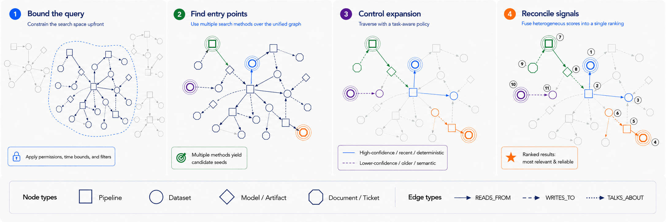
Bounding the Query. In standard vector search, filtering before or after retrieval is often an implementation choice. In a context graph, there are additional constraints. Post-filtering can create graph integrity problems. If a restricted node or edge sits between otherwise visible assets, removing it after retrieval may sever the lineage and leave the agent with disconnected fragments. It can also be inefficient, since an unconstrained traversal may touch many irrelevant historical versions before discarding them. Pushing permissions and time bounds into the graph query can avoid those problems by shrinking the traversal space upfront, but it also makes query planning, indexing, and authorization logic more complex.

Finding the Entry Point. Because construction has already collapsed the federated-search problem into a single unified index, entry-point selection can combine search methods over the graph rather than dispatching queries to separate systems. The system can reconcile semantic search over documents and tickets, keyword search over dataset and model names, exact lookup for system identifiers, and property filters over metadata such as status, classification, or size. Each method produces a different kind of candidate. The challenge is deciding which seeds are specific enough to be useful without being so narrow that they miss the relevant part of the graph.

Controlling Expansion. From each starting point, traversal has to balance recall against context size. Too little expansion misses dependencies, while too much pulls in irrelevant history, weak associations, and stale artifacts that were preserved during construction for possible future use. To manage this trade-off, traversal rules should adapt to the task and rely on the trust calibration established during construction. Live debugging, for example, calls for conservative traversal: high-confidence identity edges, runtime-validated dependencies, recent executions, and deterministic relationships. Open-ended discovery calls for broader traversal, including lower-confidence semantic edges like TALKS_ABOUT, older documents, abandoned experiments, and loosely related prior work.

Reconciling Heterogeneous Signals. Because nodes are retrieved using multiple methods, they carry fundamentally incomparable scores. The engineering challenge is signal fusion. How should the system compare incommensurate dimensions like textual relevance versus graph distance, edge confidence versus source authority, and usage frequency versus overall centrality?

Any ranking strategy has trade-offs. Fixed thresholds are simple but brittle. Learned or heuristic rerankers can combine more evidence but require calibration and feedback. LLM-based reranking can reason over richer context but adds latency, cost, and variability. The core problem is that relevance in a context graph is not purely semantic. Structurally important, well-supported assets sometimes need to outrank isolated text matches, while high-centrality generic hubs sometimes need to be downweighted.

Analytical queries

Context retrieval assembles evidence for an agent to read. Analytical querying uses the graph in its fourth role: a computational substrate. Instead of only returning context, the graph computes over topology, versions, ownership, confidence, and usage patterns to answer questions whose answers live in the structure itself.

This is different from simply returning the relevant nodes and edges and letting the agent decide what to do. Raw graph context works for small neighborhoods, but many analytical questions require deterministic computation over a much larger structure. For example, suppose the ML team wants to know which data assets are most central to product recommendation work. The answer is not stored in any single node or edge. It requires traversing from product images, review data, feature pipelines, embedding tables, training runs, notebooks, dashboards, and production services, then computing which assets sit on the most important dependency paths. An agent could inspect a sampled subgraph and make a plausible guess, but the graph layer can compute centrality directly, apply edge-confidence thresholds, respect temporal scope, enforce permissions, and return a ranked result.

Analytical queries usually fall into three groups:

• Traversal queries: Tracing lineage, following upstream and downstream dependencies, or finding all consumers of a table, model, feature set, or pipeline output.

• Structural scoring: Identifying orphaned assets, hot and cold tables, dormant models, high-centrality nodes, weakly supported relationships, or assets that act as bridges between otherwise separate workflows. These scores help agents prioritize what deserves attention instead of treating every retrieved artifact equally.

• Aggregate computation: Rolling up costs, mapping team footprints, summarizing unused data outputs, counting affected customers or sellers, or computing ownership coverage across a region of the graph.

Stable analytical queries can also be materialized back into the graph. A recurring centrality computation, for example, can become a dependency_centrality_score property on a dataset, model, or service node. A frequently used lineage traversal can become a cached dependency summary. This makes future retrieval faster and gives agents precomputed signals they can use when deciding where to look next. However, materialized analytical state introduces its own responsibilities. Derived scores and cached traversals must be refreshed, versioned, and validated against the underlying graph. Otherwise, the graph risks turning stale computations into authoritative context.

Feedback loop

Interaction is not just about reading from the graph. The graph should learn not only from source systems like Slack, Jira, Snowflake, and MLflow, but also from how people and agents use the context it retrieves.

Feedback can be explicit: an engineer accepts an agent’s suggested fix, upvotes a retrieved explanation, or corrects a mistaken dependency. It can also be implicit. Users repeatedly open the same downstream service, ignore certain retrieved documents, narrow a query’s time window, or ask follow-up questions about missing dependencies. These actions signal what the retriever got right or wrong.

The value of this feedback is that it helps close the gap between the graph’s inferred structure and the organization’s real operating state. A graph may infer that two datasets are related because they share similar names, but repeated usage can show whether that relationship is actually useful. If a weak semantic edge consistently appears in successful debugging sessions, the system can raise its confidence. If a document is repeatedly skipped, contradicted, or marked irrelevant, the system can lower its rank or prune the edge that surfaced it.

Supporting this loop makes the architecture more complex. The system needs a way to write updates back to the graph, resolve conflicts, track provenance, and weight signals by source, confidence, recency, and repetition. Not every interaction should immediately mutate durable graph state. A single skipped result may mean the result was irrelevant, or it may simply mean the user was in a hurry. A correction from a domain expert should carry more weight than a correction from a general-purpose agent.

A practical design is to separate feedback into layers. Low-confidence signals can first affect ranking and retrieval behavior without changing the underlying graph. Higher-confidence signals can update edge weights, add annotations, or create candidate relationships for later confirmation, but most durable graph changes should happen in offline batches, after the system has analyzed signals across sources. A skipped document, a successful fix, a corrected dependency, and a deployment outcome are each useful on their own, but they are far more reliable when interpreted together. Only the strongest signals, such as a human-confirmed dependency or an accepted fix tied to a successful deployment, should promote an uncertain edge into a durable graph fact.

This continuous feedback loop allows the graph to self-heal over time. It can strengthen reliable connections, turn uncertain matches into confirmed ones, identify stale relationships, and surface missing links. More importantly, it lets the context graph adapt not only to source-system updates and change events, but also to the way the organization actually uses its knowledge in practice.

Context graph vs. agentic search

As the engineering challenges discussed above illustrate, implementing a context graph is a massive undertaking. For many organizations, this raises a fair question. If we already equip capable AI agents with SQL clients, GitHub integrations, and log parsers, what does a context graph provide that an advanced agent couldn't just map out on its own?

In principle, a strong agent can traverse these systems to reconstruct context on the fly. In practice, however, treating cross-system structure as runtime work creates severe bottlenecks. The penalty for this reconstruction is paid on every single query, the resulting retrieval paths are highly non-deterministic, and recovering complex historical sequences from primary sources is simply too slow for real-time inference.

When faced with these limitations, a common industry rebuttal is that stronger future models will naturally close the gap. This is a category error. Arguing that frontier LLMs will eliminate the need for context graphs is structurally identical to arguing that faster CPUs make database indices unnecessary. Model capability is not a substitute for data infrastructure. A context graph provides what runtime search cannot: a stable data model, a unified index, an immutable memory layer, and a computational substrate. Agentic search remains an essential tool, but it belongs on top of this infrastructure rather than in place of it.

Assessing whether to make this investment requires understanding exactly where runtime search breaks down, and where the context graph provides a definitive edge. The table below summarizes the main dimensions where context graphs change agent behavior. The use cases that follow then show how those differences play out in practice for the e-commerce ML team.

In practice, these dimensions rarely show up one at a time. The next two use cases show how they interact in the ML team’s day-to-day work.

Use case 1: iterating on the production model

The objective: Improve the product recommendation model in production. This requires identifying the exact model currently serving traffic, analyzing its performance, and engineering new predictive signals for the next version.

The context reality: The codebase is full of conflicting static signals. A configuration file (config.py) hardcodes MODEL_SAVE_NAME = "saved_model2.keras". The runtime reality, however, is that the live API serves a pre-computed predictions.csv generated by an offline batch job using saved_model3.keras. Additionally, the core user feature dataset driving this model is also consumed by a successful churn prediction model built by a different team, which recently engineered a new time_since_last_click signal.

Observed agentic failure: The agent searched the repository to establish a baseline. Because configuration files look authoritative, the agent fell victim to authority bias, confidently but incorrectly diagnosing saved_model2.keras as the production model. Believing it had the right artifact, the agent then wrote custom Python scripts to scrape historical logs for performance analysis. These dynamically generated scripts were brittle, repeatedly crashing due to log schema changes. Ultimately, the agent burned massive compute resources analyzing a model that wasn’t even in production, and it failed completely to discover the successful features engineered by sibling teams.

The context graph resolution: The context graph made establishing the true baseline immediate. Because the graph tracked versions of predictions.csv alongside the explicit execution records of the notebook that generated it, it deterministically traced the live API’s inputs backward to saved_model3.keras. This runtime evidence explicitly outranked the static config.py constants, saving the agent from analyzing the wrong model. Furthermore, the agent anchored on the core user feature dataset and structurally traversed forward to discover the sibling Churn Prediction model, instantly identifying and extracting the new time_since_last_click signal to reuse.

Use case 2: building an image captioning service

The objective: Build a reusable product-image captioning service that generates natural-language descriptions for the full e-commerce catalog.

The context reality: Image captioning requires running raw images through a heavy vision encoder to create embeddings. Computing these from scratch is a costly trap. The product recommendation team already ran this exact batch job to generate visual embeddings for their model (as seen in Use case 1). Additionally, an abandoned Jupyter notebook from six months ago documents a critical pitfall. Standard cropping breaks the aspect ratio of company photos. While traditional systems often ignore failed experiments, this historical context prevents teams from repeating expensive mistakes.

Observed agentic failure: The agent found the raw product images in S3 and immediately started writing a pipeline to compute the embeddings from scratch. Operating in a stateless, isolated session, the agent’s exploratory search loop entirely missed both the recommendation team’s pre-computed BigQuery table and the old Jupyter notebook. By relying purely on semantic association rather than structural dependency, the agent wasted thousands of dollars on redundant GPU compute and repeated the exact aspect-ratio mistakes a previous engineer had already discovered.

The context graph resolution: The agent anchored on the primary S3 bucket node. Instead of writing code, it utilized structural scoring (node centrality) to traverse the downstream execution lineage. It instantly discovered the highly utilized, "hot" BigQuery table containing the exact pre-computed embeddings. Expanding its ego-graph further, it traversed a semantic edge to the older, failed Jupyter notebook. Instead of ignoring it as a failure, the agent extracted the aspect ratio insight before writing any code. By reusing existing artifacts and learning from historical failures, the agent completed the task in hours instead of days.

Escaping the rebuild loop

In April 2026, an internal Amazon document reported by Business Insider described what its authors called "AI sprawl": agents and copilots making it easier for teams to build duplicate internal tools, while also producing derived artifacts that outlived the source data they came from after that data was deleted or made private. Amazon publicly disputed parts of the document, but the underlying dynamic is exactly the cross-system reasoning failure this post has been describing: thousands of engineers across autonomous teams unable to find one another's work, and therefore likely to repeat the same mistakes. AI had lowered the cost of building so much that the cost of not finding existing context became the dominant tax. That is what organizational-scale cross-system reasoning looks like when every agent has to reconstruct enterprise state on its own.

A context graph shifts this reconstruction burden from the individual agent to the shared infrastructure. The agent stops acting like a detective reconciling contradictory artifacts and becomes a consumer of pre-resolved organizational state. The conflicts, duplicates, and rediscoveries that drove the failures above are handled at the data layer, not at inference time. Cross-system reasoning shifts from per-task reconstruction to per-task consumption.

This shift is not free. A context graph requires substantial dedicated infrastructure to continuously ingest, reconcile, and validate relationships across the enterprise. All of this architecture has to be maintained as the underlying systems evolve. The investment is justified not by company size alone, but by operational shape. It pays off when the source of truth is split across many systems, when decisions and incidents need to be reconstructed at past points in time, and when multiple teams or agents would otherwise repeat the same context reconstruction. Conversely, the graph is overkill when the data footprint is simple (a single warehouse with narrow semantic scope), when the use cases are straightforward (like basic summarization or single-turn Q&A), or when the key advantages of a context graph, such as determinism and efficiency, simply do not matter. In those cases, retrieval over a unified vector index plus targeted tool calls is usually enough.

Where the investment does fit, the value compounds. The feedback loop lets the graph self-heal: edges that prove useful in successful tasks gain confidence, while edges that are repeatedly skipped or contradicted lose it. A single graph can serve many agents across teams, so each new agent inherits the institutional memory others helped build. This is a structural answer to AI sprawl: not detecting duplication after the fact, but creating a substrate where duplication and divergence are visible when work begins.

For organizations operating across fragmented systems, the question is no longer whether agents need a map of the enterprise. It is whether we build it once or pay the cost of rebuilding it forever.